Statistical Analysis to Classify the Pass Outcomes
In this post, we will learn how to use statistical learning to build models for classifying pass outcomes. Classification is the operation of labeling a set of data into different classes, for example whether a pass from a player will be a successful or an unsuccessful pass depending on a set of particular features. The pass outcome is the dependent class variable and the features are the independent variables. Classification tasks can be either binary or multiclass.
We will again use the statsbomb open data to collect information about different kind of passes and use various classification algorithms from statistical learning literature to classify these pass outcomes. First, we will import the relevant packages:
from statsbombpy import sb # statsbomb api
import matplotlib.pyplot as plt # matplotlib for plotting
import seaborn as sns # seaborn for plotting useful statistical graphs
import numpy as np # numerical python package
import pandas as pd # pandas for manipulating and analysing data
Let us now look into the different competitions available:
comp = sb.competitions()
## credentials were not supplied. open data access only
print(comp.to_markdown())
## |    |   competition_id |   season_id | country_name             | competition_name        | competition_gender   | season_name   | match_updated              | match_available            |
## |---:|-----------------:|------------:|:-------------------------|:------------------------|:---------------------|:--------------|:---------------------------|:---------------------------|
## |  0 |               16 |           4 | Europe                   | Champions League        | male                 | 2018/2019     | 2021-04-19T17:36:05.724116 | 2021-04-19T17:36:05.724116 |
## |  1 |               16 |           1 | Europe                   | Champions League        | male                 | 2017/2018     | 2021-01-23T21:55:30.425330 | 2021-01-23T21:55:30.425330 |
## |  2 |               16 |           2 | Europe                   | Champions League        | male                 | 2016/2017     | 2020-08-26T12:33:15.869622 | 2020-07-29T05:00           |
## |  3 |               16 |          27 | Europe                   | Champions League        | male                 | 2015/2016     | 2020-08-26T12:33:15.869622 | 2020-07-29T05:00           |
## |  4 |               16 |          26 | Europe                   | Champions League        | male                 | 2014/2015     | 2020-08-26T12:33:15.869622 | 2020-07-29T05:00           |
## |  5 |               16 |          25 | Europe                   | Champions League        | male                 | 2013/2014     | 2020-08-26T12:33:15.869622 | 2020-07-29T05:00           |
## |  6 |               16 |          24 | Europe                   | Champions League        | male                 | 2012/2013     | 2020-08-26T12:33:15.869622 | 2020-07-29T05:00           |
## |  7 |               16 |          23 | Europe                   | Champions League        | male                 | 2011/2012     | 2020-08-26T12:33:15.869622 | 2020-07-29T05:00           |
## |  8 |               16 |          22 | Europe                   | Champions League        | male                 | 2010/2011     | 2020-07-29T05:00           | 2020-07-29T05:00           |
## |  9 |               16 |          21 | Europe                   | Champions League        | male                 | 2009/2010     | 2020-07-29T05:00           | 2020-07-29T05:00           |
## | 10 |               16 |          41 | Europe                   | Champions League        | male                 | 2008/2009     | 2020-08-30T10:18:39.435424 | 2020-08-30T10:18:39.435424 |
## | 11 |               16 |          39 | Europe                   | Champions League        | male                 | 2006/2007     | 2021-03-31T04:18:30.437060 | 2021-03-31T04:18:30.437060 |
## | 12 |               16 |          37 | Europe                   | Champions League        | male                 | 2004/2005     | 2021-04-01T06:18:57.459032 | 2021-04-01T06:18:57.459032 |
## | 13 |               16 |          44 | Europe                   | Champions League        | male                 | 2003/2004     | 2021-04-01T00:34:59.472485 | 2021-04-01T00:34:59.472485 |
## | 14 |               16 |          76 | Europe                   | Champions League        | male                 | 1999/2000     | 2020-07-29T05:00           | 2020-07-29T05:00           |
## | 15 |               37 |          42 | England                  | FA Women's Super League | female               | 2019/2020     | 2021-04-28T19:48:01.172671 | 2021-04-28T19:48:01.172671 |
## | 16 |               37 |           4 | England                  | FA Women's Super League | female               | 2018/2019     | 2021-04-28T19:48:01.166958 | 2021-04-28T19:48:01.166958 |
## | 17 |               43 |           3 | International            | FIFA World Cup          | male                 | 2018          | 2020-10-25T14:03:50.263266 | 2020-10-25T14:03:50.263266 |
## | 18 |               11 |          42 | Spain                    | La Liga                 | male                 | 2019/2020     | 2020-12-18T12:10:38.985394 | 2020-12-18T12:10:38.985394 |
## | 19 |               11 |           4 | Spain                    | La Liga                 | male                 | 2018/2019     | 2021-04-20T03:24:51.029365 | 2021-04-20T03:24:51.029365 |
## | 20 |               11 |           1 | Spain                    | La Liga                 | male                 | 2017/2018     | 2021-04-19T17:36:05.805404 | 2021-04-19T17:36:05.805404 |
## | 21 |               11 |           2 | Spain                    | La Liga                 | male                 | 2016/2017     | 2021-02-02T23:24:58.985975 | 2021-02-02T23:24:58.985975 |
## | 22 |               11 |          27 | Spain                    | La Liga                 | male                 | 2015/2016     | 2020-07-29T05:00           | 2020-07-29T05:00           |
## | 23 |               11 |          26 | Spain                    | La Liga                 | male                 | 2014/2015     | 2020-07-29T05:00           | 2020-07-29T05:00           |
## | 24 |               11 |          25 | Spain                    | La Liga                 | male                 | 2013/2014     | 2020-07-29T05:00           | 2020-07-29T05:00           |
## | 25 |               11 |          24 | Spain                    | La Liga                 | male                 | 2012/2013     | 2020-07-29T05:00           | 2020-07-29T05:00           |
## | 26 |               11 |          23 | Spain                    | La Liga                 | male                 | 2011/2012     | 2020-07-29T05:00           | 2020-07-29T05:00           |
## | 27 |               11 |          22 | Spain                    | La Liga                 | male                 | 2010/2011     | 2020-07-29T05:00           | 2020-07-29T05:00           |
## | 28 |               11 |          21 | Spain                    | La Liga                 | male                 | 2009/2010     | 2020-07-29T05:00           | 2020-07-29T05:00           |
## | 29 |               11 |          41 | Spain                    | La Liga                 | male                 | 2008/2009     | 2020-07-29T05:00           | 2020-07-29T05:00           |
## | 30 |               11 |          40 | Spain                    | La Liga                 | male                 | 2007/2008     | 2020-07-29T05:00           | 2020-07-29T05:00           |
## | 31 |               11 |          39 | Spain                    | La Liga                 | male                 | 2006/2007     | 2020-07-29T05:00           | 2020-07-29T05:00           |
## | 32 |               11 |          38 | Spain                    | La Liga                 | male                 | 2005/2006     | 2020-07-29T05:00           | 2020-07-29T05:00           |
## | 33 |               11 |          37 | Spain                    | La Liga                 | male                 | 2004/2005     | 2020-07-29T05:00           | 2020-07-29T05:00           |
## | 34 |               49 |           3 | United States of America | NWSL                    | female               | 2018          | 2020-07-29T05:00           | 2020-07-29T05:00           |
## | 35 |                2 |          44 | England                  | Premier League          | male                 | 2003/2004     | 2020-08-31T20:40:28.969635 | 2020-08-31T20:40:28.969635 |
## | 36 |               72 |          30 | International            | Women's World Cup       | female               | 2019          | 2020-07-29T05:00           | 2020-07-29T05:00           |
Our aim is to get access to all of Barcelona’s available pass event data in La Liga stretching from 2004/05 season to 2019/20 season. We will filter comp by setting competition_name to La Liga.
comp = comp[comp["competition_name"] == "La Liga"]
print(comp.to_markdown())
## |    |   competition_id |   season_id | country_name   | competition_name   | competition_gender   | season_name   | match_updated              | match_available            |
## |---:|-----------------:|------------:|:---------------|:-------------------|:---------------------|:--------------|:---------------------------|:---------------------------|
## | 18 |               11 |          42 | Spain          | La Liga            | male                 | 2019/2020     | 2020-12-18T12:10:38.985394 | 2020-12-18T12:10:38.985394 |
## | 19 |               11 |           4 | Spain          | La Liga            | male                 | 2018/2019     | 2021-04-20T03:24:51.029365 | 2021-04-20T03:24:51.029365 |
## | 20 |               11 |           1 | Spain          | La Liga            | male                 | 2017/2018     | 2021-04-19T17:36:05.805404 | 2021-04-19T17:36:05.805404 |
## | 21 |               11 |           2 | Spain          | La Liga            | male                 | 2016/2017     | 2021-02-02T23:24:58.985975 | 2021-02-02T23:24:58.985975 |
## | 22 |               11 |          27 | Spain          | La Liga            | male                 | 2015/2016     | 2020-07-29T05:00           | 2020-07-29T05:00           |
## | 23 |               11 |          26 | Spain          | La Liga            | male                 | 2014/2015     | 2020-07-29T05:00           | 2020-07-29T05:00           |
## | 24 |               11 |          25 | Spain          | La Liga            | male                 | 2013/2014     | 2020-07-29T05:00           | 2020-07-29T05:00           |
## | 25 |               11 |          24 | Spain          | La Liga            | male                 | 2012/2013     | 2020-07-29T05:00           | 2020-07-29T05:00           |
## | 26 |               11 |          23 | Spain          | La Liga            | male                 | 2011/2012     | 2020-07-29T05:00           | 2020-07-29T05:00           |
## | 27 |               11 |          22 | Spain          | La Liga            | male                 | 2010/2011     | 2020-07-29T05:00           | 2020-07-29T05:00           |
## | 28 |               11 |          21 | Spain          | La Liga            | male                 | 2009/2010     | 2020-07-29T05:00           | 2020-07-29T05:00           |
## | 29 |               11 |          41 | Spain          | La Liga            | male                 | 2008/2009     | 2020-07-29T05:00           | 2020-07-29T05:00           |
## | 30 |               11 |          40 | Spain          | La Liga            | male                 | 2007/2008     | 2020-07-29T05:00           | 2020-07-29T05:00           |
## | 31 |               11 |          39 | Spain          | La Liga            | male                 | 2006/2007     | 2020-07-29T05:00           | 2020-07-29T05:00           |
## | 32 |               11 |          38 | Spain          | La Liga            | male                 | 2005/2006     | 2020-07-29T05:00           | 2020-07-29T05:00           |
## | 33 |               11 |          37 | Spain          | La Liga            | male                 | 2004/2005     | 2020-07-29T05:00           | 2020-07-29T05:00           |
We see that the competion_id is 11 for all the rows. So, now, we need to collect all the values from season_id. Let us get the values:
season_ids = comp.season_id.unique()
print(season_ids)
## [42 4 1 2 27 26 25 24 23 22 21 41 40 39 38 37]
Now that we have all the values of La Liga’s season_id and that we know the competition_id, we can now get all the required pass event data. Let us get the event data from the last three seasons:
ev = {}
i = 0
for si in season_ids[:3]:
    mat = sb.matches(competition_id = 11, season_id = si)
    match_ids = mat.match_id.unique()
    for mi in match_ids:
        events = sb.events(match_id = mi)
        ev[i] = events
        i+=1
L = list(ev.values())
events = pd.concat(L)
Note that the above chunk will take quite an amount of time to complete the process of collecting the data. The reader should take some break in the meantime and go grab a cup of coffee/tea! It is recommended to store this dataset as a .csv file for later use. Now let us filter the dataset by discarding unnecessary columns and picking up those which are relevant to pass events:
E_pass = events[['type', 'pass_angle', 'pass_height', 'pass_length', 'pass_outcome', 'team']]
print(E_pass.head(10).to_markdown())
## |    |   Unnamed: 0 | type        |   pass_angle | pass_height   |   pass_length |   pass_outcome | team             |
## |---:|-------------:|:------------|-------------:|:--------------|--------------:|---------------:|:-----------------|
## |  0 |            0 | Starting XI |    nan       | nan           |     nan       |            nan | Deportivo Alavés |
## |  1 |            1 | Starting XI |    nan       | nan           |     nan       |            nan | Barcelona        |
## |  2 |            2 | Half Start  |    nan       | nan           |     nan       |            nan | Barcelona        |
## |  3 |            3 | Half Start  |    nan       | nan           |     nan       |            nan | Deportivo Alavés |
## |  4 |            4 | Half Start  |    nan       | nan           |     nan       |            nan | Barcelona        |
## |  5 |            5 | Half Start  |    nan       | nan           |     nan       |            nan | Deportivo Alavés |
## |  6 |            6 | Pass        |      3.09995 | Ground Pass   |      16.8146  |            nan | Barcelona        |
## |  7 |            7 | Pass        |     -2.25894 | Ground Pass   |      11.6516  |            nan | Barcelona        |
## |  8 |            8 | Pass        |      1.71269 | Ground Pass   |       7.77817 |            nan | Barcelona        |
## |  9 |            9 | Pass        |     -1.51327 | Ground Pass   |      19.1316  |            nan | Barcelona        |
print(len(E_pass))
## 402627
Firstly we will only keep those rows where, type is set to 'Pass' and team is set to 'Barcelona':
E_pass = E_pass[(E_pass['type'] == 'Pass') & (E_pass['team'] == 'Barcelona')]
print(E_pass.head(10).to_markdown())
## |    |   Unnamed: 0 | type   |   pass_angle | pass_height   |   pass_length |   pass_outcome | team      |
## |---:|-------------:|:-------|-------------:|:--------------|--------------:|---------------:|:----------|
## |  6 |            6 | Pass   |     3.09995  | Ground Pass   |      16.8146  |            nan | Barcelona |
## |  7 |            7 | Pass   |    -2.25894  | Ground Pass   |      11.6516  |            nan | Barcelona |
## |  8 |            8 | Pass   |     1.71269  | Ground Pass   |       7.77817 |            nan | Barcelona |
## |  9 |            9 | Pass   |    -1.51327  | Ground Pass   |      19.1316  |            nan | Barcelona |
## | 10 |           10 | Pass   |     1.27468  | Ground Pass   |       6.16847 |            nan | Barcelona |
## | 11 |           11 | Pass   |     2.50258  | Ground Pass   |      22.3002  |            nan | Barcelona |
## | 12 |           12 | Pass   |     1.31242  | Ground Pass   |      14.4807  |            nan | Barcelona |
## | 13 |           13 | Pass   |    -2.30539  | Ground Pass   |      20.8866  |            nan | Barcelona |
## | 14 |           14 | Pass   |    -0.447427 | High Pass     |      38.5996  |            nan | Barcelona |
## | 15 |           15 | Pass   |    -2.16891  | Low Pass      |      24.6854  |            nan | Barcelona |
print(len(E_pass))
## 72069
Note that, we have reduced the size of the dataset from 402627 to 72069. We see that pass_height in E_pass is a categorical column and we need to engineer this feature to give it numerical values. Let us check the the unique types in pass_height:
print(E_pass.pass_height.unique())
## ['Ground Pass' 'High Pass' 'Low Pass']
Intuition tells us that 'Ground Pass' leads to more successful passes, 'Low Pass' leads to lesser successful passes and the 'High Pass' leads to the least successful passes. We can use a look up table to assign them some numerical values. Let us create a dict object to do so:
pass_height_types = {'Ground Pass': 3, 'High Pass': 2, 'Low Pass': 1}
We will replace the entries of the pass_height column with the above numerical values from the dictionary:
E_pass_new = E_pass.replace({"pass_height": pass_height_types})
print(E_pass_new.head(10).to_markdown())
## |    |   Unnamed: 0 | type   |   pass_angle |   pass_height |   pass_length |   pass_outcome | team      |
## |---:|-------------:|:-------|-------------:|--------------:|--------------:|---------------:|:----------|
## |  6 |            6 | Pass   |     3.09995  |             3 |      16.8146  |            nan | Barcelona |
## |  7 |            7 | Pass   |    -2.25894  |             3 |      11.6516  |            nan | Barcelona |
## |  8 |            8 | Pass   |     1.71269  |             3 |       7.77817 |            nan | Barcelona |
## |  9 |            9 | Pass   |    -1.51327  |             3 |      19.1316  |            nan | Barcelona |
## | 10 |           10 | Pass   |     1.27468  |             3 |       6.16847 |            nan | Barcelona |
## | 11 |           11 | Pass   |     2.50258  |             3 |      22.3002  |            nan | Barcelona |
## | 12 |           12 | Pass   |     1.31242  |             3 |      14.4807  |            nan | Barcelona |
## | 13 |           13 | Pass   |    -2.30539  |             3 |      20.8866  |            nan | Barcelona |
## | 14 |           14 | Pass   |    -0.447427 |             2 |      38.5996  |            nan | Barcelona |
## | 15 |           15 | Pass   |    -2.16891  |             1 |      24.6854  |            nan | Barcelona |
First, we will study logistic regression for building a binary classifier model. So our pass_outcome column should be such that it gives two values: 0 for unsuccessful passes or 1 for successful passes. Let us now look into the unique entries of the pass_outcome column:
print(E_pass_new.pass_outcome.unique())
## [nan 'Incomplete' 'Out' 'Unknown' 'Injury Clearance' 'Pass Offside']
We know that in statsbomb data a pass_outcome having a nan value actually means a successful pass. So we will replace the nan values in this column with 1 and all other values with 0.
pass_outcome_types = {'Incomplete':0, 'Out':0, 'Unknown':0, 'Injury Clearance':0, 'Pass Offside':0}
E_pass_new = E_pass_new.replace({"pass_outcome": pass_outcome_types})
E_pass_new = E_pass_new.fillna({'pass_outcome':1})
print(E_pass_new.head(10).to_markdown())
## |    |   Unnamed: 0 | type   |   pass_angle |   pass_height |   pass_length |   pass_outcome | team      |
## |---:|-------------:|:-------|-------------:|--------------:|--------------:|---------------:|:----------|
## |  6 |            6 | Pass   |     3.09995  |             3 |      16.8146  |              1 | Barcelona |
## |  7 |            7 | Pass   |    -2.25894  |             3 |      11.6516  |              1 | Barcelona |
## |  8 |            8 | Pass   |     1.71269  |             3 |       7.77817 |              1 | Barcelona |
## |  9 |            9 | Pass   |    -1.51327  |             3 |      19.1316  |              1 | Barcelona |
## | 10 |           10 | Pass   |     1.27468  |             3 |       6.16847 |              1 | Barcelona |
## | 11 |           11 | Pass   |     2.50258  |             3 |      22.3002  |              1 | Barcelona |
## | 12 |           12 | Pass   |     1.31242  |             3 |      14.4807  |              1 | Barcelona |
## | 13 |           13 | Pass   |    -2.30539  |             3 |      20.8866  |              1 | Barcelona |
## | 14 |           14 | Pass   |    -0.447427 |             2 |      38.5996  |              1 | Barcelona |
## | 15 |           15 | Pass   |    -2.16891  |             1 |      24.6854  |              1 | Barcelona |
print(E_pass_new.pass_outcome.unique())
## [1. 0.]
Now that we have manipulated our data, it is time to start building the model. For doing that, we need to use the scikit-learn package that is used for predictive statistical learning with Python. the user should pip install the package to begin with. As we are going to use logistic regression to build our model, we need to call the LogisticRegression class from scikit-learn:
from sklearn.linear_model import LogisticRegression
In addition to this, we need to split our dataset into a training dataset that aids in training our classifier and a testing dataset that is used to test the accuracy of our model. So we need to call the train_test_split class from scikit-learn.
from sklearn.model_selection import train_test_split
Finally, we need to calculate the evaluation metrics of our model. So we need to import the metrics class too:
from sklearn import metrics
As pass_outcome is the column for dependent variable and the rest are the columns for the independent variables, we have to divide the dataset into dependent and independent variables in the following way:
x = E_pass_new[['pass_angle', 'pass_height', 'pass_length']]
y = E_pass_new['pass_outcome']
print(x.head(10).to_markdown())
## |    |   pass_angle |   pass_height |   pass_length |
## |---:|-------------:|--------------:|--------------:|
## |  6 |     3.09995  |             3 |      16.8146  |
## |  7 |    -2.25894  |             3 |      11.6516  |
## |  8 |     1.71269  |             3 |       7.77817 |
## |  9 |    -1.51327  |             3 |      19.1316  |
## | 10 |     1.27468  |             3 |       6.16847 |
## | 11 |     2.50258  |             3 |      22.3002  |
## | 12 |     1.31242  |             3 |      14.4807  |
## | 13 |    -2.30539  |             3 |      20.8866  |
## | 14 |    -0.447427 |             2 |      38.5996  |
## | 15 |    -2.16891  |             1 |      24.6854  |
print(y.head(10).to_markdown())
## |    |   pass_outcome |
## |---:|---------------:|
## |  6 |              1 |
## |  7 |              1 |
## |  8 |              1 |
## |  9 |              1 |
## | 10 |              1 |
## | 11 |              1 |
## | 12 |              1 |
## | 13 |              1 |
## | 14 |              1 |
## | 15 |              1 |
Here y is the outcome and x is the set of columns representing the features. Now we split the whole dataset into training and test datasets:
x_train, x_test, y_train, y_test = train_test_split(x, y, train_size=0.4, random_state = 0)
Here, the argument train_size=0.4 states that 40% of our data will be used as training data, and the argument random_state=0 ensures that the randomly selected rows that make up the training datasets are always the same every time the function is called on our original dataset.
Let us look into the training and test datasets:
print(x_train.head(10).to_markdown())
## |        |   pass_angle |   pass_height |   pass_length |
## |-------:|-------------:|--------------:|--------------:|
## |  12504 |    -2.05555  |             3 |       16.9532 |
## |  43466 |     0.57442  |             2 |       42.8823 |
## | 248698 |     2.9105   |             3 |       17.4642 |
## | 114318 |     1.91635  |             3 |       15.9424 |
## | 375561 |    -2.85014  |             3 |       20.8806 |
## | 129796 |     0.785398 |             3 |       18.3848 |
## |  43127 |     1.36116  |             3 |       14.4156 |
## | 165840 |    -2.67795  |             2 |        6.7082 |
## | 394965 |    -0.504861 |             2 |       43.4166 |
## | 158924 |    -1.10715  |             3 |       11.1803 |
print(x_test.head(10).to_markdown())
## |        |   pass_angle |   pass_height |   pass_length |
## |-------:|-------------:|--------------:|--------------:|
## | 268532 |    0.432408  |             3 |      14.3178  |
## |  76336 |   -0.922866  |             3 |      18.0602  |
## | 177139 |   -1.24905   |             2 |       3.16228 |
## | 134226 |   -2.19105   |             3 |       8.60233 |
## |  83969 |    0.18948   |             3 |      14.8661  |
## | 197188 |    1.15839   |             3 |      17.4642  |
## | 283676 |    3.07917   |             3 |      16.0312  |
## |  91742 |    0.0658676 |             3 |      37.9824  |
## | 233291 |    0.266252  |             3 |      11.4018  |
## |  91553 |    2.67795   |             3 |      11.1803  |
print(y_train.head(10).to_markdown())
## |        |   pass_outcome |
## |-------:|---------------:|
## |  12504 |              1 |
## |  43466 |              0 |
## | 248698 |              1 |
## | 114318 |              1 |
## | 375561 |              1 |
## | 129796 |              1 |
## |  43127 |              1 |
## | 165840 |              0 |
## | 394965 |              0 |
## | 158924 |              1 |
print(x_test.head(10).to_markdown())
## |        |   pass_angle |   pass_height |   pass_length |
## |-------:|-------------:|--------------:|--------------:|
## | 268532 |    0.432408  |             3 |      14.3178  |
## |  76336 |   -0.922866  |             3 |      18.0602  |
## | 177139 |   -1.24905   |             2 |       3.16228 |
## | 134226 |   -2.19105   |             3 |       8.60233 |
## |  83969 |    0.18948   |             3 |      14.8661  |
## | 197188 |    1.15839   |             3 |      17.4642  |
## | 283676 |    3.07917   |             3 |      16.0312  |
## |  91742 |    0.0658676 |             3 |      37.9824  |
## | 233291 |    0.266252  |             3 |      11.4018  |
## |  91553 |    2.67795   |             3 |      11.1803  |
Now, we will create an instance of the logistic regression model:
lr = LogisticRegression()
Next, we will train our model on the training dataset:
lr.fit(x_train, y_train)
## LogisticRegression()
Once the training is done, we will predict the outcomes of the passes on the test data:
y_predicted = lr.predict(x_test)
Yes, we have generated our predicted outcomes. To check the accuracy of our model, we use the metrics.accuracy_score() function:
accuracy = metrics.accuracy_score(y_test, y_predicted)
accuracy
## 0.8747282734378613
We see that our classification model has around 87.47% accuracy. Not bad! Next, we need a way to compare y_test and y_predicted. This is usually done by visualizing the confusion matrix or the error matrix in the following way:
error_matrix = metrics.confusion_matrix(y_test, y_predicted,labels = [0, 1])
sns.heatmap(error_matrix, annot=True, cmap = 'Blues_r', linewidths = 3, linecolor = 'red')
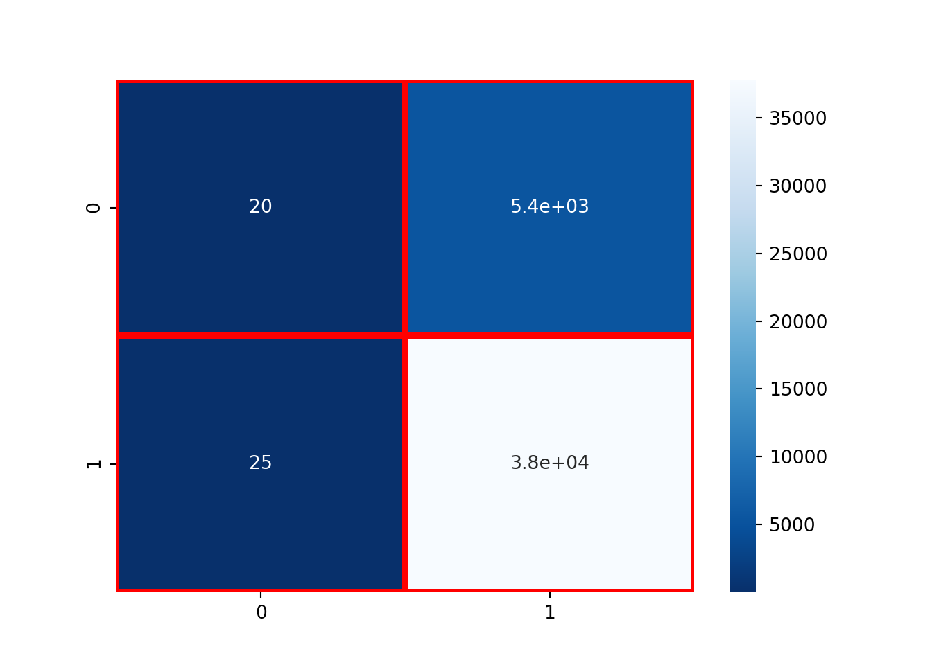
Now, from this confusion matrix we can calculate the true negatives, false positives, false negatives and true positives:
TN, FP, FN, TP = error_matrix.ravel()
print(TN, FP, FN, TP)
## 20 5392 25 37805
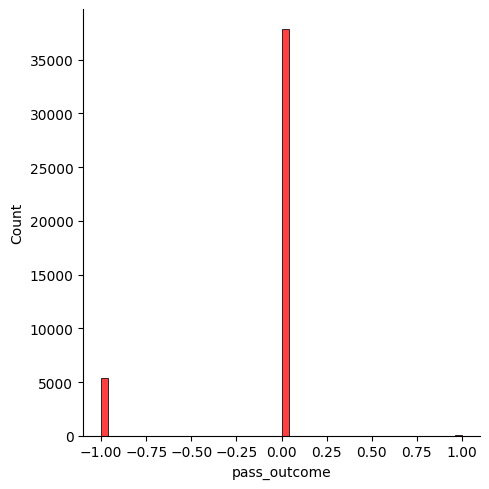
So, there are 20 true negatives, 5392 false positives, 25 false negatives and 37805 true positives to be precise. We can also confirm this by plotting a histogram to show the difference between the predicted value and the true value:
sns.displot((y_test - y_predicted), bins = 50, color = 'red')
We can finally calculate the mean absolute error:
mae = metrics.mean_absolute_error(y_test, y_predicted)
mae
## 0.12527172656213867
So, our model prediction is off by the value given by mae. Next, we will study how to perform multi-label classification on the same dataset by using another statistical learning algorithm called the Naive Bayes algorithm.
First let us clean E_pass dataset a little more by discarding those pass_outcomes which are either 'Unknown' or 'Injury Clearance'.
E_pass = E_pass[E_pass['pass_outcome'].isin(['Unknown', 'Injury Clearance']) == False]
print(E_pass.pass_outcome.unique())
## [nan 'Incomplete' 'Out' 'Pass Offside']
As we are going to work with multi-label classification, let us modify the pass_outcome_type look up table:
pass_outcome_types = {'Incomplete':0, 'Out':-1, 'Pass Offside':-2}
We will now alter E_pass by changing the pass_outcome column based on the new look up table:
E_pass_new = E_pass.replace({"pass_height": pass_height_types})
E_pass_new = E_pass_new.replace({"pass_outcome": pass_outcome_types})
E_pass_new = E_pass_new.fillna({'pass_outcome':1})
print(E_pass_new.head(10).to_markdown())
## |    |   Unnamed: 0 | type   |   pass_angle |   pass_height |   pass_length |   pass_outcome | team      |
## |---:|-------------:|:-------|-------------:|--------------:|--------------:|---------------:|:----------|
## |  6 |            6 | Pass   |     3.09995  |             3 |      16.8146  |              1 | Barcelona |
## |  7 |            7 | Pass   |    -2.25894  |             3 |      11.6516  |              1 | Barcelona |
## |  8 |            8 | Pass   |     1.71269  |             3 |       7.77817 |              1 | Barcelona |
## |  9 |            9 | Pass   |    -1.51327  |             3 |      19.1316  |              1 | Barcelona |
## | 10 |           10 | Pass   |     1.27468  |             3 |       6.16847 |              1 | Barcelona |
## | 11 |           11 | Pass   |     2.50258  |             3 |      22.3002  |              1 | Barcelona |
## | 12 |           12 | Pass   |     1.31242  |             3 |      14.4807  |              1 | Barcelona |
## | 13 |           13 | Pass   |    -2.30539  |             3 |      20.8866  |              1 | Barcelona |
## | 14 |           14 | Pass   |    -0.447427 |             2 |      38.5996  |              1 | Barcelona |
## | 15 |           15 | Pass   |    -2.16891  |             1 |      24.6854  |              1 | Barcelona |
We are going to apply Naive Bayes algorithm to build our multi-label classification model. Naive Bayes algorithms are a set of simple probabilistic algorithms built upon Bayes' theorem, assuming that all the features are independent of each other. As this assumption is naive, these methods are therefore called Naive Bayes methods. First we need to call the GaussianNB class from scikit-learn:
from sklearn.naive_bayes import GaussianNB
We will next divide our dataset into dependent and independent variables:
x = E_pass_new[['pass_angle', 'pass_height', 'pass_length']]
y = E_pass_new['pass_outcome']
print(x.head(10).to_markdown())
## |    |   pass_angle |   pass_height |   pass_length |
## |---:|-------------:|--------------:|--------------:|
## |  6 |     3.09995  |             3 |      16.8146  |
## |  7 |    -2.25894  |             3 |      11.6516  |
## |  8 |     1.71269  |             3 |       7.77817 |
## |  9 |    -1.51327  |             3 |      19.1316  |
## | 10 |     1.27468  |             3 |       6.16847 |
## | 11 |     2.50258  |             3 |      22.3002  |
## | 12 |     1.31242  |             3 |      14.4807  |
## | 13 |    -2.30539  |             3 |      20.8866  |
## | 14 |    -0.447427 |             2 |      38.5996  |
## | 15 |    -2.16891  |             1 |      24.6854  |
print(y.head(10).to_markdown())
## |    |   pass_outcome |
## |---:|---------------:|
## |  6 |              1 |
## |  7 |              1 |
## |  8 |              1 |
## |  9 |              1 |
## | 10 |              1 |
## | 11 |              1 |
## | 12 |              1 |
## | 13 |              1 |
## | 14 |              1 |
## | 15 |              1 |
Now, we split the whole dataset into training and test datasets:
x_train, x_test, y_train, y_test = train_test_split(x, y, train_size=0.4, random_state = 0)
print(x_train.head(10).to_markdown())
## |        |   pass_angle |   pass_height |   pass_length |
## |-------:|-------------:|--------------:|--------------:|
## |  24742 |    -0.214967 |             3 |      23.4395  |
## | 150862 |    -0.432408 |             3 |      14.3178  |
## | 341342 |    -0.124355 |             2 |       8.06226 |
## | 106600 |     2.14671  |             3 |       9.18096 |
## | 209720 |     1.71269  |             3 |       7.07107 |
## | 177450 |     1.15257  |             3 |      19.6977  |
## | 205081 |     0.291457 |             2 |      10.4403  |
## | 287988 |     1.3734   |             3 |       5.09902 |
## | 318663 |    -1.87668  |             3 |      19.9249  |
## | 283670 |    -1.3633   |             3 |      19.4165  |
print(x_test.head(10).to_markdown())
## |        |   pass_angle |   pass_height |   pass_length |
## |-------:|-------------:|--------------:|--------------:|
## |  84315 |    -2.10613  |             3 |      16.8585  |
## | 237632 |    -0.927295 |             1 |       5       |
## |  76289 |    -0.268841 |             3 |      10.1651  |
## |  15998 |    -2.80159  |             1 |      15.5926  |
## | 364198 |     2.14213  |             3 |      16.6433  |
## | 129666 |    -3.04192  |             3 |      10.0499  |
## | 329616 |     2.70175  |             3 |      18.7883  |
## | 133871 |    -1.73595  |             3 |      12.1655  |
## |  75295 |    -0.54172  |             1 |      13.1883  |
## | 229777 |     2.35619  |             1 |       4.24264 |
print(y_train.head(10).to_markdown())
## |        |   pass_outcome |
## |-------:|---------------:|
## |  24742 |              1 |
## | 150862 |              1 |
## | 341342 |              1 |
## | 106600 |              1 |
## | 209720 |              1 |
## | 177450 |              1 |
## | 205081 |              0 |
## | 287988 |              0 |
## | 318663 |              1 |
## | 283670 |              1 |
print(y_test.head(10).to_markdown())
## |        |   pass_outcome |
## |-------:|---------------:|
## |  84315 |              1 |
## | 237632 |              1 |
## |  76289 |              1 |
## |  15998 |              1 |
## | 364198 |              1 |
## | 129666 |              1 |
## | 329616 |              1 |
## | 133871 |              1 |
## |  75295 |              1 |
## | 229777 |              1 |
Then, we will create an instance of the Naive Bayes model:
nb = GaussianNB()
Next, we will train our model on the training dataset:
nb.fit(x_train, y_train)
## GaussianNB()
Once the training is done, we will predict the outcomes of the passes on the test data:
y_predicted = nb.predict(x_test)
After we predict the outcomes, we test the accuracy of our model:
accuracy = metrics.accuracy_score(y_test, y_predicted)
accuracy
## 0.8430598453356866
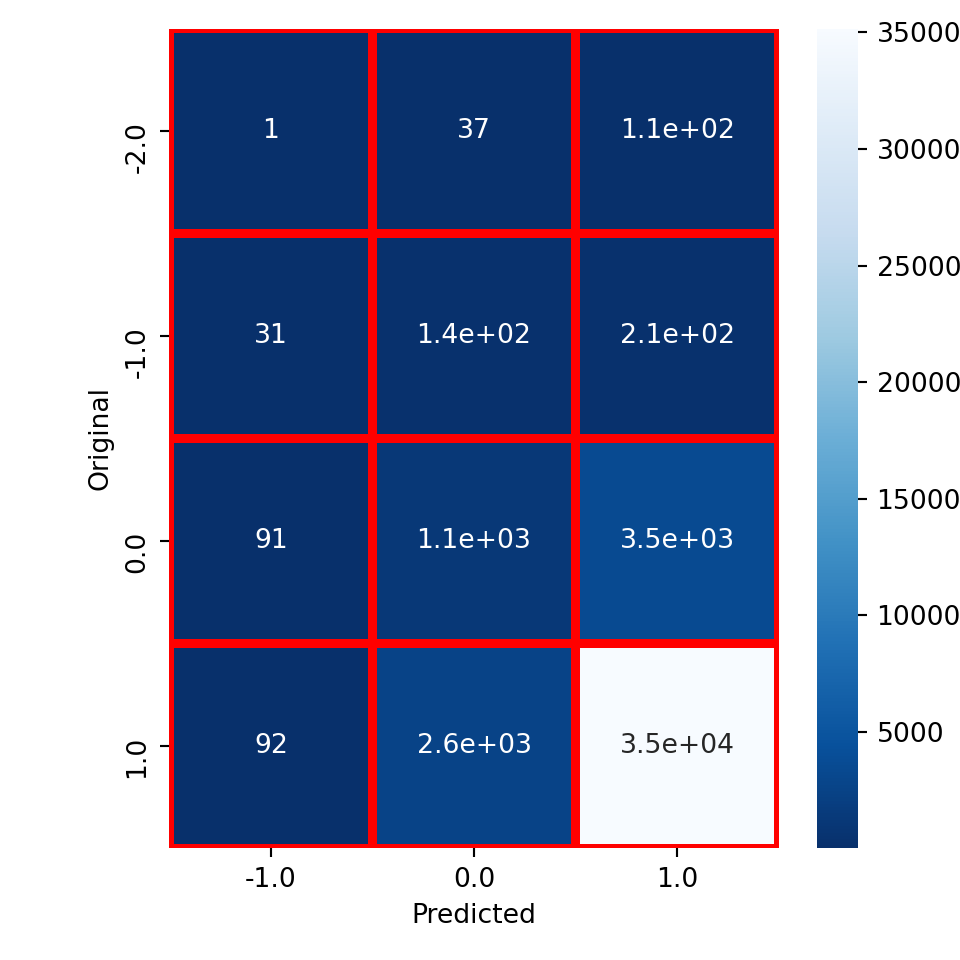
Our model has an accuracy of about 84.3%. We then compute and visualize the error matrix and calculate the values of true negatives, false positives, false negatives and true positives:
error_matrix = metrics.confusion_matrix(y_test, y_predicted,labels = [-2, -1, 0, 1])
sns.heatmap(error_matrix, annot=True, cmap = 'Blues_r', linewidths = 3, linecolor = 'red')
## <AxesSubplot:>
plt.show()

error_matrix.ravel()
## array([    0,     1,    37,   108,     0,    31,   144,   211,     0,
##           91,  1114,  3467,     0,    92,  2607, 35158], dtype=int64)
error_matrix = pd.crosstab(y_test, y_predicted, rownames=['Original'], colnames=['Predicted'])
sns.heatmap(error_matrix, annot=True, cmap = 'Blues_r', linewidths = 3, linecolor = 'red')
## <AxesSubplot:xlabel='Predicted', ylabel='Original'>
plt.show()
Finally let us visualize the difference histogram and compute the mean absolute error
sns.displot((y_test - y_predicted), bins = 50, color = 'blue')
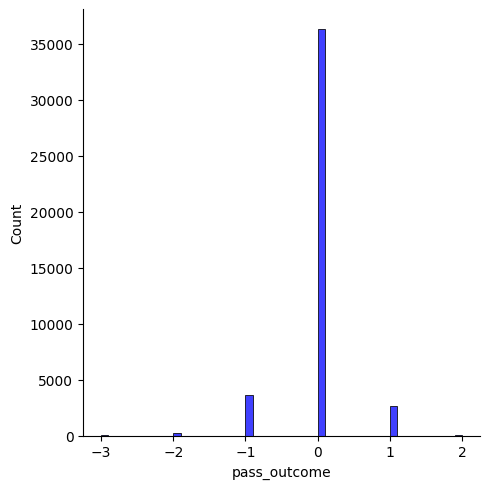
mae = metrics.mean_absolute_error(y_test, y_predicted)
mae
## 0.16985207031885
This completes our post on classifying different pass outcomes using two statistical learning algorithms, one for binary classification and the other for multi-label classification.